Queues

Published about 8 years ago

Last week we discussed stacks, the LIFO, data structure that allows us to push and pop elements onto and from it. This week we cover queues, the stack’s partner in crime.

While a stack is a Last In First Out data structure, if this doesn’t make sense to you see last weeks article, Stacks. A queue on the other hand is a First In First Out, or FIFO. This simply means that the first element to be placed in the queue is the first one to leave. In other words it’s a line.

Hurry up and wait.

So a stack has two essential methods. The “enqueue”, or place an element at the back of the line, and the “dequeue”, or remove element from the front of the line. Let’s look at an image to solidify this.

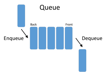
Pretty simple, right? So, lets get our hands dirty and create an implementation in Ruby.

Much like the stack we implemented in the last blog, Ruby makes implementing a queue trivial. The below implementation of a queue is really unnecessary, but for the sake of learning, is valuable.

class Queue
  def initialize
    @queue = []
  end

  def enqueue(item)
    @queue.push(item)
  end

  def dequeue
    @queue.shift
  end
end

That’s really it. Like I said above, this implementation is purely academic, serving no real purpose other than to learn how a queue works. Ruby gives us the array methods to mimic a queue without having to create the above queue class.

So now that we understand how queues work, let us consider where queues work. Anytime you need a first come, first served type of interaction, a queue is suitable.

Consider a web server that serves files to hundreds, if not thousands of users at a time. All of these users cannot be serviced at the same time, so we put the requests in line, using a queue, and serve them in the order the requests were placed. Another example is at a hardware level. A processor cannot run all processes asked of it at the same time, instead we queue up the processes and run them in order.

These are just two examples. I’m sure, with little effort, you can imagine many more. Thanks for reading along, until next week, consider the links below.

Wikipedia - Queue

Wikipedia - FIFO

Stacks

Published about 8 years ago

Continuing our journey exploring data structures and algorithms using Ruby as a means to implement them, we will now turn our attention to Stacks. If you have followed along up until now, this is going to be a piece of cake. 

What is a stack? A stack is a linear data structure, like a linked list or an array. As a matter of fact, the most common stack implementations involve either a linked list or an array as the underlying data structure. The defining quality of a stack is the fact that it is Last In First Out (LIFO). In other words the last item that was added, or “pushed”, to the stack is the first item that the stack will return, or “pop”.

So a stack has two basic methods associated with it that we hinted at above. The “push” is how we add an item to the stack. The “pop” is how we get the top element off of the stack. You can imagine a stack as pez dispenser. The first piece of pez that you insert into the dispenser is the last one you will get out of it, conversely, the last piece of candy you put in the dispenser is the first you get out. Perhaps the image below will clear up any confusion.

There is one other method that many stacks implement, the “peek”. This method allows us to see the topmost element without actually “popping” it off. It is considered optional because of the fact that is essentially just a “pop” followed by a “push” of the element back onto the stack.

Ruby makes implementing a Stack trivial. As a matter of fact, Ruby arrays give us a push and pop method built in, and Ruby’s last method is essentially a “peek”, returning the last element of the array without actually removing it. So the below implementation of a Stack feels unnecessary, and it is, but hopefully this gives you a better understanding of how a Stack works.

class Stack
  def initialize
    @stack = []
  end

  def push(item)
    @stack.push(item)
  end

  def pop
    @stack.pop
  end

  def peek
    @stack.last
  end
end

That’s it, as discussed above, this is entirely an academic, learning implementation. Since Ruby provides us with all the functionality to mimic a Stack with its Array data structure. We create a new stack on initialization which is really just an empty array. We then leverage the built in push, pop and last methods to implement the push, pop, and peek methods of the Stack class.

Stacks are not uncommon in the wild, although, working at the abstraction level that most web developers work, we don’t think of them very often. Anytime you need to retrace your steps a Stack is a handy data structure, perhaps using the back button in a browser or traversing a maze. At a hardware level Stacks allow for recursive algorithms, pushing results on the stack for use later when the recursion bubbles back up to the initial call. This can also result in the dreaded stack overflow, duh, duh, duh. At the most basic hardware level, there is only so much memory available to the stack, try to push an extra element onto the stack and you get a stack overflow, or worse, a locked up computer.

Hopefully you have a better understanding of stacks now, how they work, and what they might be used for. Thanks for reading along, I suggest taking a look at the wikipedia link below for a more in depth article on Stacks that doesn’t focus only on Ruby. Until next time.

Stack (abstract data type) - Wikipedia

Linked Lists

Published about 8 years ago

So far in our journey to better understand data structures and algorithms from a web developer’s perspective we have been focusing mostly on some basic sorting algorithms, namely insertion and merge sorts. It’s time to shift gears away from the pure algorithms and have a look at some data structures and the algorithms associated with them.

As web developers we use data structures daily, usually arrays, because, well, they are easy to use and provided to us as built in data structures in nearly every language. In this post, however, we are going to take a look at a another basic data structure, the linked list. As a matter of fact, a good understanding of linked lists is critical, from it we can build implementations of arrays, stacks, queues, etc… The node of a linked list is also the fundamental piece in more complex structures like trees. Clearly, the linked list is fundamental to computer science so lets get started.

A complete Doubly Linked List implementation in Ruby can be found at the repo below. Although in this article we will be discussing Singly Linked Lists, you can see just how simple it is to make a Double Linked List by simply adding a prev pointer.

https://github.com/SYoung82/linked-lists

What is a linked list? It is, very simply, a linear collection of elements (nodes). The most basic linked list node consists of two pieces of information, data, and a reference to the next node in the sequence. More complex versions of the linked list, such as the doubly linked list, require nodes to have more information. See the image below.

Fairly simple, right? Let’s take a look at how we might implement a node in Ruby.

class Node
  attr_accessor :value, :next, :prev

  def initialize(value)
    @value = value
  end
end

That’s it, really! We created a Node class that has both a value, which we set on initialization of an instance of the node, and a pointer called next, which will point to the next node, if it exists.
In order to manipulate a collection of these nodes we have to have an initial pointer that points to the first node. We typically call this pointer head. Keeping that in mind, let’s look at an implementation of a Linked List class in Ruby.

class LinkedList
  attr_accessor :head

  def initialize(headNode = nil)
    @head = headNode
  end
end

Again, that really is it! We create a new LinkedList class which has one attribute, it’s head, which we set to nil if it’s not provided on construction of the instance. So we can say LinkedList.new() to create a new linked list whose head points to nothing. Or, we can do something like, LinkedList.new(Node.new(1)) to create a new LinkedList whose head points to a Node whose value is 1. Cool!

That’s great and all but a data structure with no algorithms is pretty much useless. So lets create the first one to get you pointed in the right direction. We definitely need the ability to append to the list of nodes. How do we do that though with only a reference to the head node? Well, we pretty much just walk our way down the list until we reach the Node whose next is not pointing to another node and attach our new node.

def insertTail(node)
  currentNode = @head

  if currentNode == nil
    @head = node
    return self
  end

  while currentNode.next != nil
    currentNode = currentNode.next
  end

  currentNode.next = node
  return self
end

So we create a pointer, currentNode, which we use as a pointer to walk through the list until we find the Node whose next == nil then we set currentNode.next to the newNode that was passed in to the method. We could also implement methods to insert a Node at the beginning of the list or after a particular node. I’ll leave those up to you, you can see solutions here, https://github.com/SYoung82/linked-lists/blob/master/linked_list.rb.

There are numerous other methods you might be asked to implement for a linked list including delete and search. They will all use a variation of the algorithm above, in which, you walk the list looking for an element or the end, and then modify a pointer or return a node as required. I encourage you to try these out on your own. If you have any trouble you can see one possible solution here, https://github.com/SYoung82/linked-lists/blob/master/linked_list.rb. Note that this implementation is a doubly linked list, although the algorithms are essentially the same.

There are a few advantages to using a linked list over an array. Most commonly cited is the fact that a linked list dynamically increases or decreases memory usage with the addition or subtraction of nodes. Arrays on the other hand, typically require more space than is necessary to avoid having to resize every time a new element is added.

Below are a few links concerning Linked Lists a little bit more in depth. Until next time.

https://en.wikipedia.org/wiki/Linked_list

http://www.geeksforgeeks.org/data-structures/linked-list/

Merge Sort

Published about 8 years ago

If you aren’t familiar with recursion please read last weeks post, Recursion, A Prelude to Merge Sort. Done? Good, let’s jump right into things then. As promised this week we will have a go at implementing a merge sort algorithm in Ruby. This is going to test our understanding of the stuff we learned in last week’s recursion post.

The merge sort is a textbook example of a divide-and-conquer algorithm. The idea being that we “divide” the array to be sorted into two sub-arrays of half the size. Then “conquer” the problem by sorting the two sub-arrays recursively using the merge sort algorithm. Finally we combine the two sorted sub-arrays back together, producing the sorted solution. This may sound a little confusing, but it will make more sense as we move along.

The below image will hopefully clear up some confusion.

At the top of the image, we have an unsorted array. We work our way down to single element arrays by recursively calling our merge sort function. The base case, remember every recursive algorithm must have a base case, is when we reach single element arrays. Then we can start comparing elements and merging them back together. Lets take a look at the code.

def merge_sort(arr)
  if arr.length <= 1  # Base Case
    return arr
  end

  mid_pt = arr.length / 2   # Divide
  left_arr = merge_sort(arr[0, mid_pt])
  right_arr = merge_sort(arr[mid_pt, arr.length])

  sorted_arr = merge(left_arr, right_arr)  # Conquer
end

Notice, the base case, arr of size 1. Also notice the two clear steps. First, “divide” if we are not at length of 1, split the array and recursively call merge_sort again with the two new arrays. Then “conquer” by merging back together. We haven’t written the merge algorithm yet, but don’t worry, we will.

So how do we implement the merge algorithm? Its fairly straightforward, but lets step through it. By the time we first call our merge function we are down to arrays of size 1, this simplifies the work we do significantly, and also helps us wrap our heads around the algorithm a little bit easier. At this point we simply compare our two single element arrays and push them onto the sorted array in the appropriate order. Easy, right?

What little complexity that exists in the merge algorithm comes about when we start considering arrays of size larger than one. This is not terribly difficult either though. We simply repeat the above steps until either the left sub-array or the right sub-array is empty, then push whatever elements are left over onto the end of the sorted array. Lets see this in action below.

def merge(left_arr, right_arr)
  sorted = []

  until left_arr.empty? || right_arr.empty?
    if left_arr[0] <= right_arr[0]
      sorted << left_arr.shift
    else
      sorted << right_arr.shift
    end
  end

  sorted.concat(left_arr).concat(right_arr)
end

Pretty cool! We create an empty array to eventually return. Then we push elements onto that array in order until one of the two input arrays is empty. Finally we just concatenate whatever is left onto the sorted array and implicitly return it. That last line might be a little odd looking, we could rearrange it and concatenate the right array then the left array, it would make no difference, since one of the two arrays has to be empty anyway.

There you have it, a ruby implemented version of merge sort. Without diving too deep into the math lets talk about the complexity of the algorithm. Most divide-and-conquer algorithms will have a complexity of some sort of log n, there are exceptions to this rule, just like with most rules. With the merge sort we get an O(n log n). Basically the division of the arrays is an O(n) operation, and the merging of the arrays back to a final solution is an O(log n) operation. Resulting in an O(n log n) worst case. I know that is not a very satisfying analysis but the math involved in a true analysis of this algorithm is beyond the scope of this article.

Thanks for reading, below are a few links if you would like some supplemental material to study regarding the merge sort.

Merge Sort

Recursion, A Prelude to Merge Sort

Published about 8 years ago

Last week we implemented and discussed the insertion sort in Ruby. We saw that insertion sort was fairly intuitive from a human beings point of view, but as far as sort algorithms go, it was not very efficient. Rather than dive right into the merge sort this week we are going to talk about recursion, a pattern that can be found all around us and is critical to understand in order to implement the merge sort. Don’t let the name , or what you might have heard about recursion in the past scare you, it’s really not that difficult. Next week we will implement the merge sort in Ruby, but in order to do that, we are going to dive into recursion this week.

A recursive algorithm is simply an algorithm that calls itself to solve a problem in progressively simpler steps. Let’s take a look at a simple recursive algorithm that prints ‘Hello World’ n times recursively.

def HelloWorldRecursive(n)
  if(n<1)
    return
  else
    puts "Hello World"
    HelloWorldRecursive(n-1)
  end
end

Lets step through this algorithm line-by-line. Assuming we call this method like so, HelloWorldRecursive(3) . You will see on line 2 above that we first check to see if n is less than one. This critically important step in all recursive algorithms is called the base case. It’s the case or sometimes cases that trigger a recursive algorithm to exit. Without this check we would be running this algorithm endlessly. Eventually running out of memory. All recursive algorithms must have a base case, or in some situations more than one base case.

Next, starting on line 4, assuming the base case was not triggered, we begin doing some recursive work. First, we simply print Hello World to the console, simple enough. Next comes the recursion, notice on line 6, we call the method we are already in! We do this by decrementing n by one. This is also critically important. If we didn’t decrease n, we would never reach our base case, and be stuck in an infinite loop.

Ultimately, this is a very contrived example that could have been solved much more easily with a simple loop. However, it illustrates the two critical pieces involved when designing a recursive algorithm.

• A recursive algorithm must have a base case that allows the algorithm to end.
• A recursive algorithm must manipulate the data in question in some way so as to eventually trigger the base case.

Without both of the above requirements an infinite loop is inevitable, which, no doubt, is not the desirable outcome.

Hopefully that silly, simplified example helped explain the basics of recursion in a way that clears up any confusion you might have had. Let’s solidify that knowledge a bit by trying solving a problem that actually lends itself a little bit better to recursion, factorials.

What is a factorial you might be asking, or you might not, if you know what a factorial is already. For those of you that don’t let’s have a quick look. Very basically the factorial of a number, n, is n multiplied by all the numbers less than n down through 1. More formally, n! = n * (n-1) * (n-2) * … * 2 * 1. For example 4! = 4 * 3 * 2 * 1 = 24.

Maybe you are already seeing the recursive pattern. We can solve 3! by finding out what 3 * 2! is. We can then solve 2! by finding out what 2 * 1! is. But wait 1! is 1. Ahh, we have found our base case. So let’s take a crack at coding this.

def factorial(n)
  if n == 1
    return 1
  else
    return n * factorial(n - 1)
  end
end

This pattern should look very familiar to our Hello World recursive algorithm above. We start by checking our base case, if n == 1 then we simply return 1 because we know that 1! is one. Otherwise we call our factorial method, recursively, and ask it what n * factorial( n — 1 ) is. This fulfills our second requirement for a recursive algorithm stated above. By removing 1 from n for each recursive call of factorial() we know that eventually n will equal 1 and our recursive algorithm will begin to return those results. The image below might help clear up how these return statements work.

{:height="30px" width="30px"}

Note that the above image illustrates an algorithm that checks for a base case of n == 0, the result is the same though since 1 * 1 = 1.

Hopefully, recursion is now a little less enigmatic. This was a very simple study in recursion, meant mostly for web developers and other less math intensive groups of programmers. Recursion is a simple idea, that is made complex by the fact that it is not very intuitive to us as human beings. Recursive patterns often don’t jump out at us like some other patterns do. That being said, recursion is everywhere in computer science, from merge sort to binary trees and beyond. Thanks to our newfound knowledge in recursion we can tackle the merge sort next week. See you then.

Recursion (computer science)

Factorial