Implementing an Undirected Graph in Ruby

Published almost 8 years ago

Last time we met we discussed the concept of Graphs in CS. In a very general way we talked about what a Graph is, the differences between Directed and Undirected Graphs, and some of the more common categories of Graphs you might encounter in the wild. If you haven’t read that article, or need to brush up before moving on, you can check it out here.

Today I’m going to have a look at implementing a very basic Undirected Graph in Ruby. We will save the traversals and other algorithms for next time. For now our focus will be solely on implementing a Graph class.

There are several ways to do this, including using an adjacency list or an adjacency matrix. I’ve decided to use an adjacency list implementation. Mostly because it makes the most sense to me, and is probably the simplest way to implement a Graph data structure.

So, what is an adjacency list? It’s simply a list of nodes that are adjacent to a given node. Take the simple undirected, cyclic Graph shown below.

In this graph, each node would have an adjacency list associated with it. Each of those adjacency lists would have two Nodes in it.

• Node a → adjacent to [ b, c]
• Node b → adjacent to [a, c]
• Node c → adjacent to [a, b]

That’s all there is to it, we just need to keep track of the list of Nodes that are connected to a given Node. Let’s implement a Node class that does this.

class Node

  attr_reader :value

  def initialize(value)
    @value = value
    @adjacent_nodes = []
  end

  def add_edge(adjacent_node)
    @adjacent_nodes << adjacent_node
  end

end

There you have it, our Node class using an adjacency list. It looks a lot like the Nodes we have used in the past for Linked Lists and Trees. The main differences being that it is instantiated with an empty list representing the adjacent Nodes, and it has a function, add_edge, that allow us to connect two Nodes.

Next step is to implement a Graph class that uses our new Node class. There are several ways to do this as well. We could keep track of the Nodes in the Graph using a List, or better yet a Set to ensure unique Nodes. However, I have elected to use a hash. Mainly because this allows us to keep a list of Nodes that will have keys based on their value. This allows us to quickly find a Node in the Graph. Check it out below.

class Graph

  def initialize
    @nodes = {}
  end

  def add_node(node)
    @nodes[node.value] = node
  end

  def add_edge(node1, node2)
    @nodes[node1].add_edge(@nodes[node2])
    @nodes[node2].add_edge(@nodes[node1])
  end

end

A few things to note. First the add_node method uses the value of the node to create the key in the @nodes hash and sets it equal to the node passed to it. This method could obviously benefit from some checks to see if a Node value already exists in the @nodes hash. For simplicity and demonstration purposes I have left that out.

Another thing to note is the add_edge method. Since we are implementing an Undirected Graph, we need to add two edges. One from node1 to node2 and vice-versa.

That’s really all there is to it. Next time comes the fun part. How do we traverse a Graph efficiently? Much like Tree traversals we can do this in a Depth-first way or in a Breadth-first way. Throw in weighted edges and you have an even more complex problem. Check out some of the reading below until next time when we implement some of these traversals.

Adjacency List - Wikipedia

Graph Traversal - Wikipedia

Graphs

Published almost 8 years ago

Our journey has taken us far. We started off with basic search algorithms and recursion. Soon we moved on to some basic data structures like Linked Lists, Stacks and Queues. Lately our focus has been on Trees, including Binary Search Trees and methods to traverse them. We haven’t exhausted Trees by a long shot, perhaps we will circle back around and take a deeper dive but for now it’s time to move on.

What’s next you might be asking, actually, you probably aren’t asking that at all since you read the title of this post. Graphs are the next logical step in our journey, since a Tree is a very specific type of Graph. In fact, a Tree is an Undirected Graph that has no cycles. This may not make sense right now but we will discuss these terms shortly.

A Graph is an abstract data type in computer science that has an entire field of study associated with it, called graph theory. As such, we won’t be able to cover every detail regarding Graphs.

Graphs have the same basic components as Trees, Nodes and Edges or Directed Edges. This makes sense, since a Tree is just a very specific type of Graph.

There are two broad types of Graphs:

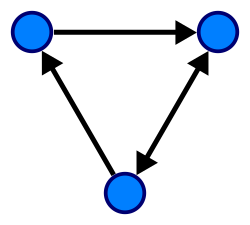
• Directed Graph — A Directed Graph is one whose Edges have direction. These directions can be one or two ways and are often called Directed Edges. See the example below.

• Undirected Graph — As it’s name implies, an Undirected Graph is one in which the edges have no direction.

Graphs may also contain cycles, or not. For example the sequence of Nodes from the Example 2 above, 4–5–2–3–4, is a cycle because the first Node is reachable from itself. There are several other cycles in this Graph as well, 5–1–2–5, is another example. Also 3–4–5–1–2–3.

A cycle graph is a Graph that is a cycle in it’s entirety. The below image is an example of the most basic Cycle Graph. Notice how each Node has degree 2, that is it each Node has two Edges emanating from it. This is true of all Cycle Graphs.

A Graph my also be a Complete Graph. A Complete Graph is one in which each Node is connected to all other Nodes. In the image below notice how there are 5 Nodes and each Node has degree of 4. All Nodes in a Complete Graph will have degree of, # Nodes - 1.

One last category of Graph worth mentioning is a Weighted Graph. A Weighted Graph is one in which a value is assigned to each Edge. These graphs are common in many types of CS problems, including shortest path problem which you are probably familiar with thanks to Google Maps or Waze.

That’s a pretty quick and dirty overview of Graphs. Next time we will start to implement a graph data structure and some of the algorithms associated with it. Some of those algorithms worth considering are adding and removing Nodes, adding and removing Edges, and testing whether two Nodes are neighbors, just to name a few.
Below is some further reading material covering some of the topics we talked about in this post as well as some more advanced topics we didn’t cover. Until next time and thanks for reading along.

Graph (abstract data type) - Wikipedia

Directed Graph - Wikipedia

Graph (discrete mathematics) - Wikipedia

Travelling Salesman Problem - Wikipedia

Tree Traversals

Published almost 8 years ago

The past few posts we have been exploring Trees. We talked about what a Tree data structure is, generally, and some of the terminology common to all trees in this post. Then we dove a little deeper and implemented a Binary Search Tree (BST) in this article. Surely we now know everything there is to know about Trees, right? Not really. We could probably write a whole series of articles over the course of a year discussing the different types of Trees and the algorithms associated with them. None of that matters though, if we don’t have a way of searching through the Nodes of a Tree, which leads to the topic du jour.

A Tree Traversal is simply an algorithm that allows us to visit each Node in a Tree, once, and only once. This can be done in multiple ways, but all ways have several steps in common. For each Node in the Tree you must:

• Determine whether a left Subtree or Node exists, if so recursively traverse it.
• Determine whether a right Subtree or Node exists, if so recursively traverse it.
• Handle the Node itself.

These steps can be done in different orders and the order in which these steps are completed determine in which order the Nodes of the Tree are traversed.

Pre-Order Traversal

A pre-order traversal does the above steps in the following order:

• Handle the current Node
• Traverse the left Subtree
• Traverse the right Subtree

This is best seen in the following diagram:

If we printed the value of each Node given the above Tree, the result would be ‘F, B, A, D, C, E, G, I, H’.

In-Order Traversal

An in-order traversal does the steps in the following order:

• Traverse the left Subtree
• Handle the current Node
• Traverse the right Subtree

Like so:

Which would result in this output: ‘A, B, C, D, E, F, G, H, I’.

Post-Order Traversal

You can probably guess in what order a post-order traversal accomplishes it’s tasks:

• Traverse the left Subtree
• Traverse the right Subtree
• Handle the current Node

Since these traversals are so similar we will not implement all of them. Instead I will implement the In-Order Traversal, and leave the rest to you for self-study if you choose. The below code assumes we are working with the BST structure we built in the last post.

def inorder(root)
  # Traverse left subtree
  if root.left
    inorder(root.left)
  end

  # Handle current node
  puts root.key

  # Traverse right subtree
  if root.right
    inorder(root.right)
  end
end

There it is, easy peasy. Implementing the other two is as simple as rearranging the above code. These algorithms are known as Depth-First Searches or DFS, due to the fact that they traverse as deep into the Tree as possible before returning and going to the next sibling.

A DFS is not the only way to traverse a tree though. There is also the concept of Breadth-First Search or BFS which looks something like this:

Resulting in this output: ‘F, B, G, A, D, I, C, E, H’

This is most commonly accomplished by using a Queue to push the children onto in order to keep track of future nodes to visit. For example we would start at root node, F, and push nodes B and G onto the Queue. After we are done with F we pop off the B and push its children onto the Queue, A and D. Now G is at the top of the Queue, we pop it off and continue this process until the Queue is empty something like this:

def dfs(root)
  q = [root]

  until q.empty?
    # Get the first node off of the queue
    current_node = q.shift

    # Check if the current_node has children and push them onto the
    # back of the queue
    if current_node.left
      q.push(current_node.left)
    end
    if current_node.right
      q.push(current_node.right)
    end

    # Print the current node
    puts current_node.key
  end
end

Good thing we covered Queues a few weeks back, eh? As you can see, fairly straightforward. We use an until loop to check if the queue is empty. Make sure to prime the queue with the root of the tree so that you don’t start with an empty queue. Then we push any children of the current Node onto the queue in order from left to right. Finally print the Node’s key value. Repeat the process until there are no more Nodes left in the Queue.

Hopefully this has shed some light on the concept of tree traversals. We have really only scratched the surface here. These concepts get more complex when we consider applying them to not just Trees but Graphs as well. Check out the links below for some further reading. Until next time.

Tree traversal - Wikipedia
Depth-first search - Wikipedia
Breadth-first search - Wikipedia

Binary Search Trees

Published almost 8 years ago

You down with BST? Yeah, you know me. Your not down with BST’s you say? Well get ready, your about to be. Last week we talked about Trees in general. This week we are going to narrow our focus and look at Binary Search Trees. So if you need to brush up on Trees in general you can do that here.

A Binary Search Tree, BST from here on out, is simply a tree with the additional property that it’s keys are in sorted order. That is, any Nodes or sub-trees on the left branch of a Node are less than the Node and any Nodes or sub-trees on the right branch of a Node are greater than the Node. See the picture below for clarification.

Notice how all the values to the left of the Root Node, 8, are less than 8 and all the values in the right sub-tree are greater than 8. This property holds for all sub-trees of the Tree as well. This single property, allows for speedy search, insert and delete methods, all three of which have average runtimes of O(log n).

Let’s get started writing some code. First off we need to implement a Node class. It should have a value and pointers to left and right nodes:

class Node
  attr_accessor :key, :left, :right

  def initialize(key)
    @key = key
    @left = nil
    @right = nil
  end
end

Pretty straightforward, our class initializer simply sets the value of the Node and the left and right pointers are set to nil.

Next, we should implement the BST class. This will also be fairly simple, as far as initialization goes. We are simply going to create a root that is set to nil. Now that’s great and all, but we can’t really do anything with it, so we will also implement an insert method at the same time which will allow us to insert Nodes into our new BST class.

class BST
  attr_accessor :root

  def initialize
    @root = nil
  end

  def insert(key)
    insert_node(@root, key)
  end

private

  def insert_node(current_node, key)
    if current_node.nil?
      current_node = Node.new(key)
    elsif key < current_node.key
      insert_node(current_node.left, key)
    elsif key > current_node.key
      insert_node(current_node.right, key)
    end
  end
end

A few things to note here. The insert method delegates to a private method, insert_node. The real work is done in the insert_node method, which compares the value that needs to be inserted to the current_node, if it is less than, we recursively call insert_node on the left child and vice-versa if it is greater, until we find an empty Node, at which point we insert a new Node.

Great, so we can build out a BST by simply creating a new BST with BST.new. The we insert nodes one by one with the insert method, passing it a key value. The next step is to implement a search method that will allow us to traverse the BST and determine if a Node with a certain key value exists.

class BST
  attr_accessor :root

  def initialize
    @root = nil
  end

  def insert(key)
    insert_node(@root, key)
  end

  def search(key)
    find_node(@root, key)
  end

private

  def insert_node(current_node, key)
    if current_node.nil?
      current_node = Node.new(key)
    elsif key < current_node.key
      insert_node(current_node.left, key)
    elsif key > current_node.key
      insert_node(current_node.right, key)
    end
  end

  def find_node(current_node, key)
    if current_node.nil?
      return nil
    end

    if current_node.key == key
      return current_node
    elsif key < current_node.key
      find_node(current_node.left, key)
    elsif key > current_node.key
      find_node(current_node.right, key)
    end
  end
end

Much like we did with the insert method, we delegate to a private method called find_node. This method starts out checking for two potential base cases, either the current_node is nil, in which case we return nil, or the current_node.key is equal to the key we are searching for, in that case we found what we are looking for and return it. Otherwise we recursively traverse the tree based on whether the key we are looking for is less than or greater than the current_node.key , just like we did in the insert method. This is a pattern you are going to see over and over in Trees. Since Trees are a recursive structure, we typically traverse them recursively.

Finally, we will implement a delete method. This is slightly more challenging than the insert and search methods. Once we find the Node we are looking for there are basically three cases to consider.

• The node has no children
• The node has either a left child or a right child
• The node has both right and left children

The first two are fairly straightforward. If the Node has no children we simply remove it. If the Node has only one child we remove the Node and replace it with its child. If the Node has two children we find it’s next successor in the Tree. This Node can be found by taking the right sub-tree and finding the minimum value in it. See the image below again.

In the instance we want to remove the Node whose value is 3, we would find its successor. To do this we would find the smallest value in its right sub-tree. In other words we go to the right child, the Node whose value is 6 and then traverse the Tree to the left until we find a leaf node, which is the Node whose value is 4. We then replace the 3 with 4 and remove the leaf Node. Let’s see the code.

class BST
  attr_accessor :root

  def initialize
    @root = nil
  end

  def insert(key)
    insert_node(@root, key)
  end

  def search(key)
    find_node(@root, key)
  end

  def delete(key)
    delete_node(@root, key)
  end

private

  def insert_node(current_node, key)
    if current_node.nil?
      current_node = Node.new(key)
    elsif key < current_node.key
      insert_node(current_node.left, key)
    elsif key > current_node.key
      insert_node(current_node.right, key)
    end
  end

  def find_node(current_node, key)
    if current_node.nil?
      return nil
    end

    if current_node.key == key
      return current_node
    elsif key < current_node.key
      find_node(current_node.left, key)
    elsif key > current_node.key
      find_node(current_node.right, key)
    end
  end

  def delete_node(current_node, key)
    if current_node.key == key
      remove_node(current_node)
    elsif current_node.key < key
      delete_node(current_node.left, key)
    elsif current_node.key > key
      delete_node(current_node.right, key)
    end
  end

  def remove_node(node)
    # Case 1: No children
    if node.left.nil? && node.right.nil?
      node = nil
    # Case 2: One child
    elsif node.right.nil? && !node.left.nil?
      node = node.left
    elsif node.left.nil? && !node.right.nil?
      node = node.right
    else
      node = replace(node)
    end
  end

  def replace(node)
    node.value = successor(node.right)
    node.right = update(node.right)
  end

  def successor(node)
    if !node.left.nil?
      successor(node.left)
    end

    return node.key
  end

  def update(node)
    if !node.left.nil?
      node.left = update(node)
    end

    return node.right
  end
end

So there is a lot of new code here, let’s go through it. Like before the delete method is simply an interface method, that delegates to delete_node. delete_node should look familiar it simply traverses the tree searching for the node to be deleted, much like we did with the insert and search methods. Once we find it we call the remove_node method which evaluates the three methods we discussed above.

If the Node has no children it simply sets it to nil. If it has only one child it sets it to that child. Finally, if it has two children we call the replace method using the Node’s right child. The replace method takes advantage of the successor and update methods to find the next successor, and update the Nodes appropriately.

This is really only the most basic implementation of a BST. I encourage you to look into traversals: in-order, pre-order, and post-order. Perhaps extend the code above to print out the tree using these traversal methods. You can also consider implementing a method that returns the height of your tree, whether or not the tree is balanced, or the number of Nodes in the tree. The possibilities are endless. Thanks for reading, below are some further study resources. Until next time.

Binary search tree - Wikipedia
Binary Search Tree | Set 1 (Search and Insertion) - GeeksforGeeks

Trees

Published almost 8 years ago

Of course we all know the old saying, “Trees, trees, the musical fruit…”. That doesn’t look quite right, oh well. We have made some serious progress in our quest to better understand CS basics from a web developers perspective. We’ve implemented Merge and Insertion Sorts. We’ve delved into data structures like Linked Lists, Stacks, and Queues. Now it’s time to climb out way up into Trees. There won’t be any coding in this post, there is simply too much information to cover and understand before we actually implement any kind of tree, whether it be a Binary Tree, Binary Search Tree, Red-Black Tree, N-ary Tree or any other type. Don’t worry if those names don’t make sense to you now, they will, after we cover the basics.

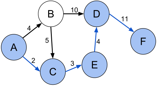
So what is a Tree in computer science? Very simply, a Tree is a data structure made up of Nodes and Edges that does not have a cycle. Ok, so what does that mean? Let’s break it down. We are familiar with Nodes thanks to linked lists, nothing has changed. A node simply contains a value or data and a link or links to other Nodes. An Edge is the link between two nodes. Makes sense, what does it mean to not have a cycle though? Well a Cycle is a path of Edges and Nodes in which a Node is reachable from itself. Take a look at the image below.

The collection of nodes (A, B, C, …) is cyclic, that is, it contains a loop. Notice how node B can be reached by following the path created by B -> C -> E -> D -> B. This collection is therefore NOT a Tree. Keeping that in mind let’s look at another image.

This is a Tree. Specifically, this is a Binary Tree. A Binary Tree is simply a Tree whose Nodes contain at most 2 children. Wait a minute, what are children? That’s a good question, let’s define some of the terminology used when talking about Trees. Keep the above image in mind while we do this.

• Root — The topmost Node in a Tree. In the example above the Node whose value is 8 .
• Edge — A connection between one node and another. The arrows in the image above.
• Child — A Node which is directly connected to another Node when moving away from the Root. Nodes 3 and 10 are Children of Node 8 above. Node 13 is a Child of Node 14 as well.
• Parent — A Parent is the opposite of a Child. The Parent of Node 1 is Node 3. Any Node in the Tree will have only one Parent.
• Sibling — A group of Nodes that have the same Parent. Nodes 1 and 6 are siblings, they have a common parent Node 3.
• Leaf — A node with no Children. Nodes 1, 4, 7, and 13 are Leaf Nodes.

Let’s take some of this terminology and talk about the characteristics of Binary Trees. A Binary Tree, as mentioned above is a Tree whose Nodes have at most 2 Children. The example image above is an example of a Binary Tree. Binary Trees have the interesting property that they have one less Edge than they have Nodes. The image above has 9 Nodes and 8 Edges. This is true of all well formed Binary Trees. Cool!

Binary Trees are also recursive in nature. The subtrees are similar to the Tree in the sense that they have a Root and potentially, that Root has at most two Children, who can themselves be the Root of a subtree. In the coming weeks as we start to implement these data structures and the algorithms to manipulate them you will see that recursion is everywhere. So if you are a little rusty on recursion go back and freshen up here.

We can also classify Binary Trees based on some of their characteristics.

• Full Binary Tree — A Tree where every node has either 0 or 2 children.
• Complete Binary Tree — A Tree where every level is completely filled, except for the last. In the last level all Nodes are as far left as possible. (Note: The Full Tree below is also a Complete Tree, it simply doesn’t need to have a last level that isn’t completely filled due to the number of nodes.)
• Binary Search Tree — A Binary Search Tree is a Binary Tree that its order in such a way that every Left Child’s value is less than it’s Parent’s Value, and every Right Child’s value is greater than it’s Parent’s Value. (Neither of the two examples below are BSTs, notice the Left Child of the Root Node is greater than the Root, that is 2 > 1. The example above that we used for defining a Tree and it’s terminology is a BST.)

That’s a lot to wrap your head around if you have never seen Trees before. Make sure you have a good understanding of this to ensure a good foundation moving forward into implementation. Below are some additional links to further your knowledge.

Tree (data structure) - Wikipedia
Binary tree - Wikipedia
Binary search tree - Wikipedia